Alexis Kruzicki - Data Visualization 1

Code

ncdc_temp <- read_csv('https://bcdanl.github.io/data/ncdc_temp_cleaned.csv')

Code

date_selected <- as.Date(c("0000-01-01", "0000-04-01",
                                            "0000-07-01",
                                            "0000-10-01",
                                            "0000-12-31"
                                            ))
df <- filter(ncdc_temp, date %in% date_selected)
p <- ggplot(data = ncdc_temp,
            mapping = 
              aes( x = date,
                   y = temperature ) )

p + geom_line( aes( color = location ),show.legend = F) +
  geom_point(data = df) +
  labs(x = "month") +
  scale_x_date(breaks = date_selected,
               date_labels = "%b")

Code

p_1 <- ggplot(data = ncdc_temp,
            mapping = 
              aes(x = temperature, 
                  y = month))
p_1 + geom_boxplot(
  fill = "grey"
) + 
  labs(x = NULL) + 
  coord_flip()

Code

library(ggridges)

p <- ggplot(data = ncdc_temp,
            mapping = 
              aes(x = temperature, 
                  y = month))
p + geom_density_ridges(alpha = 0.3, fill = "blue")

Code

cars <- mtcars

c<- ggplot(cars, aes(disp, mpg)) +
        geom_point(aes(color = hp))
c + labs(x= "displacement")+ labs(y= "fuel efficiency")

Code

popgrowth_df <- read_csv(
  'https://bcdanl.github.io/data/popgrowth.csv')

popgrowth_df %>% arrange(popgrowth, state)

# A tibble: 51 × 7
   region    division           state          pop2000  pop2010 popgrowth   area
   <chr>     <chr>              <chr>            <dbl>    <dbl>     <dbl>  <dbl>
 1 Midwest   East North Central Michigan       9938444  9883640  -0.00551 56539.
 2 Northeast New England        Rhode Island   1048319  1052567   0.00405  1034.
 3 South     West South Central Louisiana      4468976  4533372   0.0144  43204.
 4 Midwest   East North Central Ohio          11353140 11536504   0.0162  40861.
 5 Northeast Middle Atlantic    New York      18976457 19378102   0.0212  47126.
 6 South     South Atlantic     West Virginia  1808344  1852994   0.0247  24038.
 7 Northeast New England        Vermont         608827   625741   0.0278   9217.
 8 Northeast New England        Massachusetts  6349097  6547629   0.0313   7800.
 9 Midwest   East North Central Illinois      12419293 12830632   0.0331  55519.
10 Northeast Middle Atlantic    Pennsylvania  12281054 12702379   0.0343  44743.
# ℹ 41 more rows

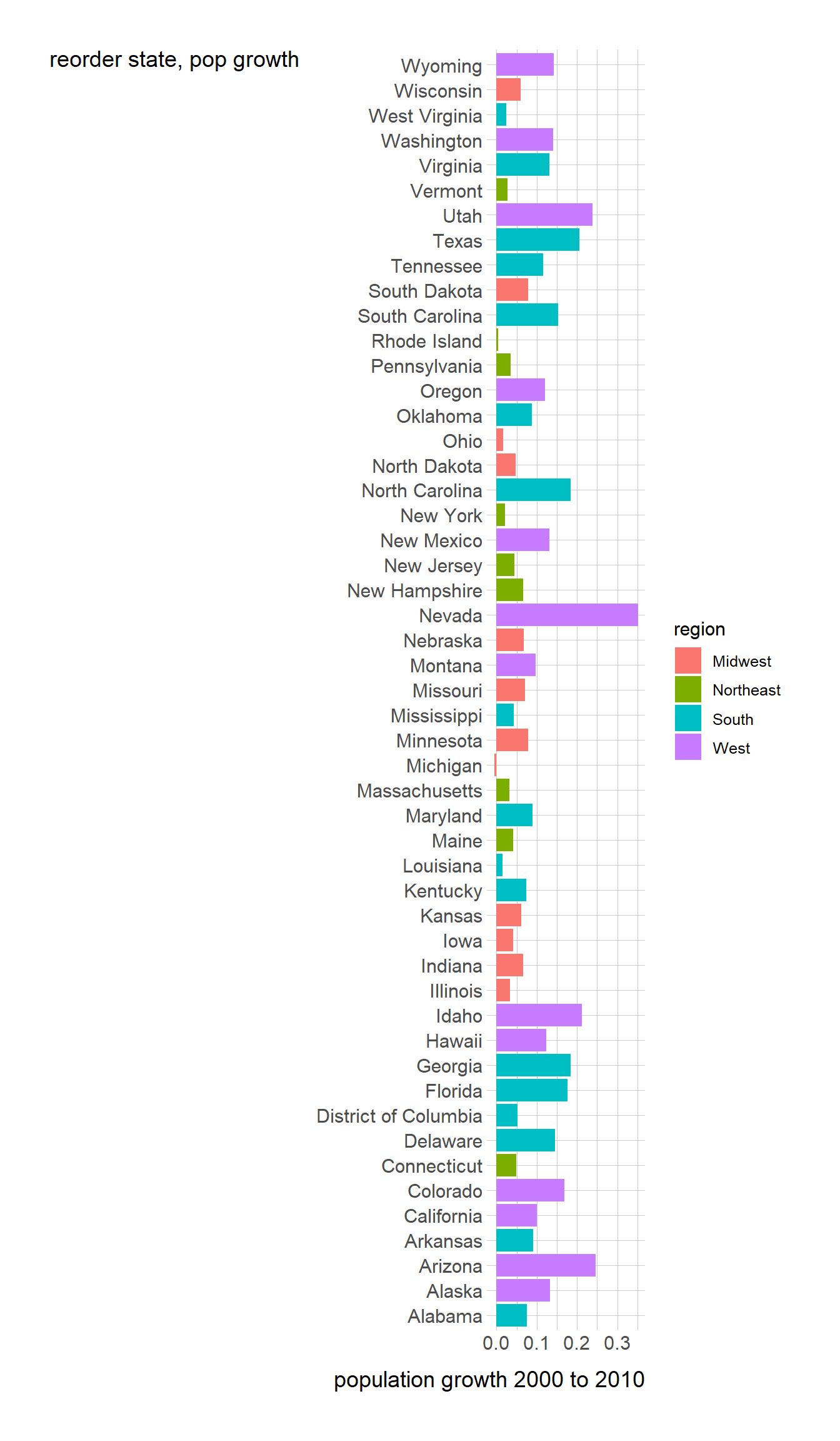
Code

pg<- ggplot(popgrowth_df, aes(state, popgrowth, fill = region)) +
        geom_bar(stat = "identity", position = "dodge") +
        coord_flip()

pg + labs(y= "population growth 2000 to 2010")+ labs(x= "reorder state, pop growth")

Code

male_Aus <- read_csv(
  'https://bcdanl.github.io/data/aus_athletics_male.csv')

ma<- ggplot(male_Aus, aes(x=height, y= pcBfat, group=sport)) +
  geom_point(aes(shape=sport, color= sport))

ma + labs(x= "height(cm)")+ labs(y= "% body fat")

Code

titanic <- read_csv(
  'https://bcdanl.github.io/data/titanic_cleaned.csv')

ggplot(titanic, aes(x=age, fill=sex)) + geom_density(alpha=0.25)

Code

cows_filtered <- read_csv(
  'https://bcdanl.github.io/data/cows_filtered.csv')

ggplot(cows_filtered, aes(x=butterfat, fill=breed)) + geom_density(alpha=0.25)

--- title: "Data Visualization 1" author: "Alexis Kruzicki" date: "2024-02-21" categories: [ code, data-visualization] execute: warning: false message: false toc: true --- ```{r} #| include: false library(knitr) library(rmarkdown) library(tidyverse) library(skimr) library(ggthemes) library(hrbrthemes) theme_set(theme_ipsum()+ theme(strip.background =element_rect(fill="lightgray"), axis.title.x = element_text(angle = 0, size = rel(1.5), margin = margin(10,0,0,0)), axis.title.y = element_text(angle = 0, size = rel(1.5), margin = margin(0,10,0,0)) ) ) ``` ```{r} ncdc_temp <- read_csv('https://bcdanl.github.io/data/ncdc_temp_cleaned.csv') ``` ```{r} date_selected <- as.Date(c("0000-01-01", "0000-04-01", "0000-07-01", "0000-10-01", "0000-12-31" )) df <- filter(ncdc_temp, date %in% date_selected) p <- ggplot(data = ncdc_temp, mapping = aes( x = date, y = temperature ) ) p + geom_line( aes( color = location ),show.legend = F) + geom_point(data = df) + labs(x = "month") + scale_x_date(breaks = date_selected, date_labels = "%b") ``` ```{r} p_1 <- ggplot(data = ncdc_temp, mapping = aes(x = temperature, y = month)) p_1 + geom_boxplot( fill = "grey" ) + labs(x = NULL) + coord_flip() ``` ```{r} library(ggridges) p <- ggplot(data = ncdc_temp, mapping = aes(x = temperature, y = month)) p + geom_density_ridges(alpha = 0.3, fill = "blue") ``` ```{r} cars <- mtcars c<- ggplot(cars, aes(disp, mpg)) + geom_point(aes(color = hp)) c + labs(x= "displacement")+ labs(y= "fuel efficiency") ``` ```{r} #| fig-height: 12 popgrowth_df <- read_csv( 'https://bcdanl.github.io/data/popgrowth.csv') popgrowth_df %>% arrange(popgrowth, state) pg<- ggplot(popgrowth_df, aes(state, popgrowth, fill = region)) + geom_bar(stat = "identity", position = "dodge") + coord_flip() pg + labs(y= "population growth 2000 to 2010")+ labs(x= "reorder state, pop growth") ``` ```{r} male_Aus <- read_csv( 'https://bcdanl.github.io/data/aus_athletics_male.csv') ma<- ggplot(male_Aus, aes(x=height, y= pcBfat, group=sport)) + geom_point(aes(shape=sport, color= sport)) ma + labs(x= "height(cm)")+ labs(y= "% body fat") ``` ```{r} titanic <- read_csv( 'https://bcdanl.github.io/data/titanic_cleaned.csv') ggplot(titanic, aes(x=age, fill=sex)) + geom_density(alpha=0.25) ``` ```{r} cows_filtered <- read_csv( 'https://bcdanl.github.io/data/cows_filtered.csv') ggplot(cows_filtered, aes(x=butterfat, fill=breed)) + geom_density(alpha=0.25) ```